Satellite Image Segmentation with Deep Learning

Project Goal
To develop a deep learning model (specifically, a U-Net variant) that segments satellite images into distinct classes (e.g., buildings, water, vegetation, roads, land, and unlabeled areas).

Welcome to this repository! Below, you will find an overview of how I prepared the data, built the model, trained it, and validated my results. I will also take a peek at interesting code snippets, along with short examples that (hopefully) keep you as amused as a caffeinated hamster.

---

Table of Contents

1. Overview of the Dataset
2. Data Preprocessing
3. Model Architecture
4. Loss Function & Metrics
5. Training & Validation
6. Results & Visualization
7. Future Work

---

Overview of the Dataset

The dataset consists of satellite tiles, each containing corresponding images and masks:

• Images are .jpg files containing RGB channels.
• Masks are .png files with assigned color codes for the different classes (building, land, road, vegetation, water, unlabeled).

For sanity checks, I read the files and discovered the usual suspects:

['image_part_001.png', 'image_part_002.png', 'image_part_003.png', ... ]

I also realized that each tile might have images of slightly different sizes. Since neural networks are picky about consistent input dimensions, I decided to patchify them into smaller squares, such as 256×256 or 512×512.

Fun fact: The reason I “patchify” large images is similar to how pizza is sliced. You don’t want to feed the entire pizza into your mouth all at once. Also, slicing helps ensure each piece is uniformly sized—makes the ML pipeline quite digestible.

---

Data Preprocessing

1. Image Patch Creation

I use patchify to split each large tile into non-overlapping 256×256 patches. Then:

image_patch_size = 256
patched_images = patchify(image, (image_patch_size, image_patch_size, 3), step=image_patch_size)

Because not all tiles’ dimensions are multiples of 256, I further cropped the images so that the width and height align nicely with our chosen patch size.

2. Normalization & Transformations

• MinMaxScaler: I normalized image pixel intensities into a [0,1] range.
• One-Hot Encoding for Masks:
  • I mapped each RGB color in the mask to an integer (e.g., water → 0, land → 1, road → 2, etc.).
  • I then expanded these labels into a categorical (one-hot) format with 6 classes.

labels_categorical_dataset = to_categorical(labels, num_classes=total_classes)

Thus, each label becomes a 6-dimensional vector.

Short Example: If a pixel belongs to class land, its label might look like [0, 1, 0, 0, 0, 0]. If it’s unlabeled, the label might be [0, 0, 0, 0, 0, 1].

---

Model Architecture

I adopt a U-Net-style architecture tailored for multi-class segmentation. Below is a quick summary:

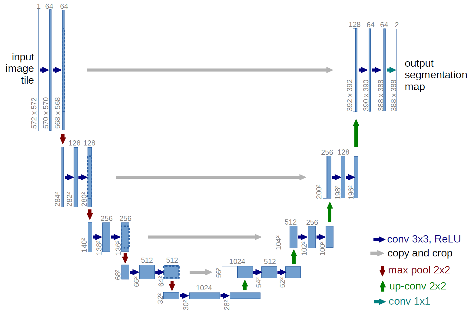
1. Downsampling/Encoder: Convolution → ReLU → Dropout → MaxPooling.
2. Upsampling/Decoder: Transposed Convolution → Concatenate with corresponding encoder layer → Convolution.
3. Final Output: Conv2D(n_classes, (1,1), activation="softmax") for multi-class classification.

def multi_unet_model(n_classes=5, image_height=256, image_width=256, image_channels=1):
    # Encoding Path
    c1 = Conv2D(16, (3, 3), activation="relu", kernel_initializer="he_normal", padding="same")(inputs)
    c1 = Dropout(0.2)(c1)
    c1 = Conv2D(16, (3, 3), activation="relu", kernel_initializer="he_normal", padding="same")(c1)
    p1 = MaxPooling2D((2, 2))(c1)

    c2 = Conv2D(32, (3, 3), activation="relu", kernel_initializer="he_normal", padding="same")(p1)
    c2 = Dropout(0.2)(c2)
    c2 = Conv2D(32, (3, 3), activation="relu", kernel_initializer="he_normal", padding="same")(c2)
    p2 = MaxPooling2D((2, 2))(c2)

    c3 = Conv2D(64, (3, 3), activation="relu", kernel_initializer="he_normal", padding="same")(p2)
    c3 = Dropout(0.2)(c3)
    c3 = Conv2D(64, (3, 3), activation="relu", kernel_initializer="he_normal", padding="same")(c3)
    p3 = MaxPooling2D((2, 2))(c3)

    c4 = Conv2D(128, (3, 3), activation="relu", kernel_initializer="he_normal", padding="same")(p3)
    c4 = Dropout(0.2)(c4)
    c4 = Conv2D(128, (3, 3), activation="relu", kernel_initializer="he_normal", padding="same")(c4)
    p4 = MaxPooling2D((2, 2))(c4)

    # Bottleneck
    c5 = Conv2D(256, (3, 3), activation="relu", kernel_initializer="he_normal", padding="same")(p4)
    c5 = Dropout(0.2)(c5)
    c5 = Conv2D(256, (3, 3), activation="relu", kernel_initializer="he_normal", padding="same")(c5)

    # Decoding Path
    u6 = Conv2DTranspose(128, (2, 2), strides=(2, 2), padding="same")(c5)
    u6 = concatenate([u6, c4])
    c6 = Conv2D(128, (3, 3), activation="relu", kernel_initializer="he_normal", padding="same")(u6)
    c6 = Dropout(0.2)(c6)
    c6 = Conv2D(128, (3, 3), activation="relu", kernel_initializer="he_normal", padding="same")(c6)

    u7 = Conv2DTranspose(64, (2, 2), strides=(2, 2), padding="same")(c6)
    u7 = concatenate([u7, c3])
    c7 = Conv2D(64, (3, 3), activation="relu", kernel_initializer="he_normal", padding="same")(u7)
    c7 = Dropout(0.2)(c7)
    c7 = Conv2D(64, (3, 3), activation="relu", kernel_initializer="he_normal", padding="same")(c7)

    u8 = Conv2DTranspose(32, (2, 2), strides=(2, 2), padding="same")(c7)
    u8 = concatenate([u8, c2])
    c8 = Conv2D(32, (3, 3), activation="relu", kernel_initializer="he_normal", padding="same")(u8)
    c8 = Dropout(0.2)(c8)
    c8 = Conv2D(32, (3, 3), activation="relu", kernel_initializer="he_normal", padding="same")(c8)

    u9 = Conv2DTranspose(16, (2, 2), strides=(2, 2), padding="same")(c8)
    u9 = concatenate([u9, c1])
    c9 = Conv2D(16, (3, 3), activation="relu", kernel_initializer="he_normal", padding="same")(u9)
    c9 = Dropout(0.2)(c9)
    c9 = Conv2D(16, (3, 3), activation="relu", kernel_initializer="he_normal", padding="same")(c9)

    outputs = Conv2D(n_classes, (1, 1), activation="softmax")(c9)
    model = Model(inputs=[inputs], outputs=[outputs])

    return model

Fun aside: Think of the U-Net architecture like a symmetrical hourglass. It pinches down the image data in the middle, then tries to reconstruct it back up. If it were a building, it’d be the wonkiest hourglass-shaped tower in the city—yet excellent at capturing context on the way down and reconstructing finer details on the way up.

---

Loss Function & Metrics

1. Dice Loss

Helps handle data imbalance. Intuitively measures how well the predicted segmentation overlaps with the true mask.

2. Categorical Focal Loss

Helps focus the model on classes that are harder to predict.

3. Total Loss

I sum Dice Loss and Focal Loss (weighted 1:1) to get the final objective.

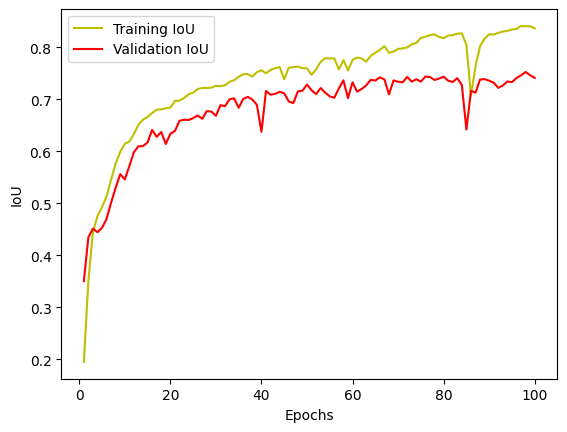
4. Jaccard Coefficient (IoU)

Used as an additional metric to evaluate overlap between the predictions and ground truth masks.

Quick Example: If your predicted building region has 80% overlap with the real building region, your IoU for that class is 0.8.

---

Training & Validation

I split the data into 85% training and 15% validation. The training happens for 100 epochs on mini-batches of 16 images at a time:

model.compile(optimizer="adam", 
              loss=total_loss, 
              metrics=["accuracy", jaccard_coeff])

history_a = model.fit(X_train, y_train,
                      batch_size=16,
                      epochs=100,
                      validation_data=(X_test, y_test),
                      shuffle=False)

Each epoch logs:

• Training Loss, Accuracy, IoU
• Validation Loss, Accuracy, IoU

Training Curves

After training, I plot the loss and IoU curves:

plt.plot(epochs, loss, 'y', label='Training loss')
plt.plot(epochs, val_loss, 'r', label='Validation loss')
plt.legend(); plt.show()

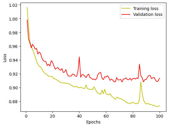
A typical learning curve shows that both training and validation losses decrease over time (with some fluctuations, of course).

---

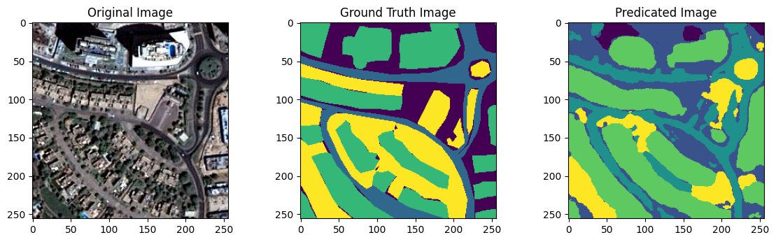
Results & Visualization

I generate segmentation predictions on X_test. Then, I compare them to the ground truth:

y_pred = model.predict(X_test)
y_pred_argmax = np.argmax(y_pred, axis=3)
y_test_argmax = np.argmax(y_test, axis=3)

Random example visualization:

test_image = X_test[some_random_number]
prediction = model.predict(np.expand_dims(test_image, 0))
predicted_image = np.argmax(prediction, axis=3)[0, :, :]

Below is a conceptual side-by-side:

+------------------------+----------------------+----------------------+
|      Original Image    |   Ground Truth Mask |   Predicted Mask    |
+------------------------+----------------------+----------------------+
| (a pretty satellite    |  (RGB-coded classes)|  (integer-labeled   |
|   tile from above)     |                     |    mask, or a color |
|                        |                     |    map if preferred)|
+------------------------+----------------------+----------------------+

Often, the predicted mask looks quite similar to the ground truth. Small discrepancies might remain around boundary regions or less frequent classes.

---

Future Work

1. Data Augmentation: Adding random flips, rotations, or color jitters could yield more robust models.
2. Larger Patch Size: Sometimes 512×512 patches allow the network to capture more context. (Though it may require more GPU memory.)
3. Advanced Architectures: Experiment with Transformers or state-of-the-art architectures such as SegFormer or DeepLabv3.

Potential Funny Side Quest: Provide a short “Where’s Waldo?” twist—where the “Waldo” class is set to a unique color, and I see if the network can find him from a tiny satellite vantage point.

---

Model Saving

Finally, I save the trained U-Net model as an .h5 file (with a friendly note that the HDF5 format is somewhat “legacy” in modern Keras land):

model.save("satellite_segmentation_full.h5")

---

Credits

Credits to https://youtu.be/UBzMgr6yfpw?si=-FtLpQw6NTSbYVFJ for inspiring the project.

Contact

Please feel free to open an Issue or Pull Request if you have any suggestions or discover potential improvements.